



Executive Summary
In the aftermath of the 2008 financial crisis, investor ownership of single-family homes increased substantially. Investors owned about 13% of detached single-family homes in 2006 and more than 17% in 2014. As families regrouped and started purchasing more homes again, investors were seen as competition—pushing the price of homes out of the reach of families. Currently, legislation in state houses across the country and a provision in the recently passed federal comprehensive housing bill aim to limit investor ownership of single-family homes.
In research for a new working paper, my co-authors and I discovered that the idea that investors are pricing families out of homes couldn’t be more wrong. New laws that limit investor activity will add more disruptions to the American housing market, which has already had more than enough disruptions.
Several basic observations led us to question the common fears about investors. First, the average real US home price dropped by more than 20% from 2006 to 2014, when investors piled into single-family housing. When prices rose again to new highs after 2014, investor market share declined just as sharply. Investors own about the same portion of detached single-family homes today as they did in 2007. Prices have dropped when investors were buyers and risen when investors were sellers. The aggregate data couldn’t be clearer. Families outbid investors for homes.
Yet, in cross-sectional studies, rising investor ownership has been found to be associated with moderately rising home prices. This was a mystery we thought was worth solving. The important beginning point for solving it was (1) to try to comprehensively account for the reason that home prices declined so much after 2006 when investors entered the market, and (2) to account for the low prices at which investors bought into the market.
The answer to point 1 is mortgage access. Mortgage access was sharply and permanently curtailed in 2008. There had been a subprime lending boom that heated up in late 2003 and essentially ended in 2007. But, after that, in the panic and chaos of the Great Recession, the federal mortgage agencies further tightened access to mortgages compared to decades of norms. In many markets in the interior of the country, home prices had never been particularly elevated, but the sudden rug pull of mortgage access in 2008 caused them to drop to levels well below historical norms or the cost to build new homes. The neighborhoods that were most sensitive to mortgage access collapsed the most, and those were the neighborhoods that investors bought into. Their rising market share was entirely the result of more supply of homes available to investors when potential homeowners were suddenly locked out. That is why prices were collapsing when investors were buying.
And, that is related to the second point. If an investor buys a house at a 25% discount, and the value of that house then increases by 5%, a researcher could find that the arrival of investors was associated with a 5% price increase, when really the arrival of investors, all told, was associated with a 20% price decrease.
That is the story of single-family investors over the past 20 years. In the aggregate, they are always and everywhere associated with moderating prices. When homeowner demand collapsed, investor buyers kept prices from falling even more. When homeowners returned, homeowners were the source of demand that drove home prices higher.
In two-way causality tests, we found that throughout the period since 2006, investors have always tended to buy into neighborhoods where prices had declined relative to other neighborhoods. Before 2012, when investors were buying, prices continued to fall. That makes sense. Prices were falling where homeowners were missing, and where a lot of them were missing, investors were struggling to gather the capital to buy all the homes that needed buyers. They couldn’t completely stop the decline.
After 2012, when home prices were rising again, more investors were associated with moderately rising prices, which partially retraced the losses that had come before the investors. Yet, even that is an understatement of the moderating role investors were playing. All homes are owned by investors or homeowners, so rising investor market share means lower homeowner market share. So, you could also say that declining homeowner market share after 2012 has been associated with rising prices.
What could that mean? It is because investors were continuing to buy homes where homeowners were missing. After 2012, families bought homes in the neighborhoods where families could still get mortgage funding. They bought some of those homes from investors, and those investors then looked for homes in neighborhoods that were still priced at discounts and bought homes there.
Investors have systematically sold out of neighborhoods where family owners could buy homes at normal prices and bought into neighborhoods where families can no longer attain mortgages, and homes continue to be undervalued. This is why investor activity has been associated with rising prices. They are only buying where prices are discounted and rising prices are called for.
Investors have been an important factor moderating prices and reverting prices to the norm, from above and below. This is the opposite of competing for homes or taking homes from families. They have systematically bought homes that needed buyers and sold homes where families were buying.
Since families with mortgage funding always outbid investors for existing homes, renters have been the main losers. Since the return of homeowner demand has poached so many homes out of the rental market, excess rent inflation over the past decade has accumulated at unprecedented rates. Essentially no renter households formed from 2016 to 2023. There are nearly 10 million missing renter households today because the homes they need haven’t been constructed. That gap will only be slowly closed by new construction. To close that gap, those potential renters will need investors. A law that limits investors will make markets for homeowners more volatile, but, more importantly, it will turn the loss of renter households from a temporary condition to a permanent condition. Anti-investor laws are anti-renter laws.
The essay that follows goes into the history that led to our current condition and summarizes the working paper where my co-authors and I conducted more sophisticated statistical tests on these questions.
Introduction
At the turn of the 21st century, the American housing market went through a lending and building boom and then, after a financial crisis in 2008, a bust. While the building boom didn’t return, high prices did. Before prices re-inflated, however, the literature on the causes of the boom was already being written, and that literature has largely assumed that the lending boom, the building boom, and the price bubble were inextricably linked. Now we know that they aren’t. Prices have risen without a lending or building boom.
The literature is due for an update. In hindsight, what looked like normal prices in 2012 according to national home price indexes, were actually an average of homes in coastal metropolitan areas like New York City and Los Angeles, where home values are perpetually inflated because building booms are legally blocked by local land use regulations, and homes in cities across the country where newly tightened mortgage access had pushed prices so low that builders couldn’t profitably compete with new homes. The pieces that added up to that normal US average home price were not normal at all—in fact, they were less normal than they had ever been before.
Adjusted for inflation, residential real estate in the U.S. doubled in value from 1998 to 2006, reaching $45 trillion, then fell back to $31 trillion in 2012. Today, U.S. residential real estate is worth nearly $60 trillion, even though real net investment in new homes since 2012 has amounted to less than $5 trillion. The period surrounding 2008 was infamously volatile, prefaced by financial exuberance and followed by employment and financial collapse and dislocation. A lending boom did temporarily inflate American home prices in 2006, but the cyclical impulse was not nearly as large as it seemed. The persistently high home prices in places like New York City and Los Angeles had permanently raised average American home values. In 2026, home prices aren’t cyclically elevated, even though American homes are now worth $60 trillion. Prices in many cities are now inflated because of short supply.
On the topic of housing, this complicates the basis for analysis. What was the correct, cyclically neutral, economically sustainable value of American real estate? $45 trillion in 2006? $31 trillion in 2012? Or nearly $60 trillion today? This is an important question and one that is easy to get wrong, because if one of those values serves as a reasonable benchmark, the others are clearly very wrong. And, as noted above, $31 trillion in 2012 is a terrible benchmark, when existing homes in much of the country were selling at prices so low that new construction dried up.
Somebody has to own every house, and so, initially, the pre-existing market of small-scale investors bought homes that families were selling either because of foreclosures or because of life changes that coincided with a time when other families who traditionally would have purchased their homes were now locked out of access to mortgages.
A nascent market of large-scale investors buying single-family homes eventually developed after the 2008 crisis. In the markets with the largest number of missing homeowners, small scale investors didn’t have enough capital to keep prices from continuing to collapse. Eventually the discounts were so deep that large institutions took an interest in the market.
Since real estate values started rising again after 2012, there have been concerns that the market power of these new home buyers could be a reason housing has become more expensive and homeownership less attainable. A review of what American housing markets looked like 20, 50, or 100 years ago might shed light on that concern.
Historically, outside small niche markets, there was no market for neighborhoods of new homes built as rentals, and no large firms engaged in the ownership and management of single-family rental homes. Historically, a number of small-scale multi-unit home types were common, often housing the owner and a few tenants. Over the course of the 20th century, those home types fell out of favor with municipal planners—urbanists have come to call those housing types the “missing middle”—and housing became more bifurcated between large apartment properties, which were generally rented, and single-family detached homes, which were generally owned. By the turn of the century, about six out of seven single-unit homes were owned by the families that lived in them, and the rest were rental units owned by small-scale investors. Conversely, about six out of seven multi-unit homes were rental units, which, of course, considering the size of the properties, were owned by firms.
The Great Recession was associated with millions of foreclosures and a decline in homeownership, but homeownership had begun to decline several years before the crisis. Yet only after 2010 did large institutional investors begin to dip their toes into the single-family rental market. They began making sizable investments after 2011, but the American housing market is very large. In 2026, institutional investors that own more than 100 homes, as a group, still own less than 1% of all single-family homes and about 5% of single-family rentals. Nevertheless, their presence has raised concerns about market concentration.
The question itself, “What effects do investors have on single-family housing markets?” presumes an active causality. It presumes that an external change in investor behavior has shifted their capital allocation decisions, thereby altering housing markets.
Can we be certain of that? Maybe investors were reacting to changes in home prices. Did the investors’ demand for the main input (homes) of the product they sell (shelter services) increase, driving up the cost of that input? Or, did other changes in the housing marketplace lower the prices of homes so that investors with stable characteristics and expectations purchased a higher quantity of homes under new conditions?
And, what conditions should we consider to be cheap—the $31 trillion market, a $60 trillion market, or somewhere in between? Were the conditions under which investors bought those homes associated with a stable, functional marketplace? Or were they temporarily pushed too high or low by “irrational exuberance” or financial discombobulation?
There is unanimity that there was a “housing bubble” before 2008 and that prices in cities like Phoenix or Orlando after 2005 were bound to correct downward. Great care would need to be taken to account for the causes of home price trends after 2005 from those temporarily elevated prices to sustainable levels. They mostly declined because they were too high.
What about when U.S. residential real estate was only worth $31 trillion in 2012? In many locations, those prices were at least as unsustainably far from a reasonable price as they had been in 2005, when prices were high, yet they have generally been accepted as a normal reflection of stable supply and demand. Benchmarking against 2012 yields results just as spurious as benchmarking against 2005 would.
In a nutshell, a necessary preliminary question is “Did the housing market come to investors, or did investors come to the housing market?” This has important policy implications because the answer to that question points to diametrically opposed policy needs. If they came to the market, then it might someday be reasonable to worry about market concentration or to consider public policy reforms that create a more satisfying balance between the availability of affordable rental homes that investors provide, versus the availability of owned homes that families might also sometimes prefer.
If investors entered the housing market, there may be reasonable motivations to ensure that every family has fair access to it. If the market came to investors, they are more likely to be filling a need that they are best suited to fill, and it may be more appropriate to encourage them to be more active.
The existing literature has tended to treat large investors, a priori, as active agents of change because of the size and scale of the capital they deploy. When they are net buyers, they are “taking homes away from families,” yet when they are net sellers, families are not modeled as “taking homes away from” corporations or renters. The temptation to treat size as an unquestionable signal of agency and power has led researchers to proceed with causal analysis before carefully testing these important preliminary questions.
Below, I will attempt to ask those questions more carefully to establish agency more clearly. The 21st-century housing market has been unusually volatile. Knowing precisely what trends and temporary dislocations to control for is exceptionally important. And with the potential for such diametrically opposed conclusions, precision is key to understanding the forces currently shaping the housing market and to shaping appropriate future policies. It is especially important at the moment. Congress considered effectively ending large-scale investment in single-family rental housing in debates around the recently passed “21st Century ROAD to Housing Act”. At the same time, bills are being introduced in states around the country that would limit investor activity in one form or another, and they are starting to pass.
In a new analysis with two co-authors, we have found strong evidence that investors routinely buy homes where homeowners are selling and sell homes where willing and able homeowners are buying. Their market presence has been so strong that they haven’t just acted to moderate rising home prices where homeowner demand is rising. They systematically disinvest from those neighborhoods and reinvest in neighborhoods that remain undervalued.
Historical Evidence of Market Power in Housing
A broad view of market norms in US housing from the Great Depression to today suggests a strong imbalance of market power. Before 2008, new single-family housing markets were dominated by families. The Census Bureau conducts a quarterly survey of Starts and Completions by Purpose and Design. It includes several categories of home types, including multi-family units built for sale (condos) or for rent (apartments), and single-family homes built for sale, or by their owner or a contractor. The market for new homes built directly for the rental market has historically been so consistently small that the survey, which has been conducted quarterly since 1974, has no tracked category for it.
New single-family homes had only one target market—homeowners. There were a few investors in single-family housing, but they tended to buy older, depreciating units rather than new ones. And there were no large investors. Over the decades, in the Census-tracked housing sales activity before 2008, not once did a large investor outbid a small investor or a family for a single-family home. And small investors never bought new single-family homes in large quantities.
The history of the US housing market strongly suggests that market power is in this order:
- Families with cash or access to mortgage funding
- Small investors
- Large investors
- Families without cash or access to mortgage funding
This runs counter to our intuitions about size and power, but the empirical historical record leaves little to debate.
In fact, the way concerns about housing are framed implies this strong power imbalance. Market power comes from both an ability and a willingness to pay. Unfortunately, families that don’t have access to a large amount of cash or to mortgage funding lack the ability to pay for homes.
Investors are feared because families value homeownership. When a large investor buys a home, it seems like it is stealing the dream of homeownership from some family. Talk of the American Dream implies great value in ownership. Families with the ability to pay for homes dominated the 20th-century housing market because their willingness to pay for them was high. There is value in being one’s own landlord.
In the 20th century and today, access to funds for families is the primary factor moving them from the bottom of the market power list to the top. Funded families have market power because homeownership has value. The market power that investors have is a product of how much families are willing to pay to rent a home versus how much they are willing to pay to own it.
In this way, the idea that investors might be pricing families out of homeownership is internally incoherent. Investors would be willing to pay more than families for homes only if families’ preferences led to higher rental yields for investors. On the other hand, investors must own homes when families are unable to buy them because they lack access to credit which would allow them to pay for the benefit of homeownership.
On a cost basis, research from Dick Oosthuizen with the Federal Reserve Bank of Philadelphia suggests that homeowner families have the advantage in competition for buying homes. He found that before the Great Recession, the cost of ownership for mom & pop investors was 21% higher than for owner-occupiers and 35% higher for institutional investors (here defined more broadly as any private corporate [non-individual] owner).
He finds that as the institutional owners expanded their footprint and achieved economies of scale, they improved their costs. By 2015, mom-and-pop investors still had ownership costs 21% higher than owner-occupiers, while institutional investors had improved their costs so that they were only 24% higher than owner-occupiers. But institutional investors were still in third place.
Oosthuizen finds that the expansion of institutional investors provided a price floor after 2008. The reduction in costs, by his estimate, raised the price floor by 1.6 percentage points, while the more efficient management of rental properties lowered the average rents for renter households.
While the economics of large-scale single-family investment improved, the 20th-century ranking of market power as home buyers remained the same: (1) Families with mortgage access or cash, (2) small investors, (3) large investors, then (4) families without capital.
Large investors continue to play the role of market supporters, filling in the gap where other owners are lacking, and providing housing for renters where the other sources of tenancy are out of reach, or where scale is necessary for the product type (either in large, multi-unit buildings, or in single-family neighborhoods managed as a single property).
Viewing recent markets carefully, home values were generally unsustainably low by 2012, when large investors initiated their first positions. If they had been more competitive with lower costs, they would have been in a position to replace missing homeowners more robustly, and they would have helped to prevent home prices from collapsing so far.
More investors, both large and small, would have been associated with less volatility in housing markets, and their arrival has never been systematically associated with inflated prices—only a return to normal.
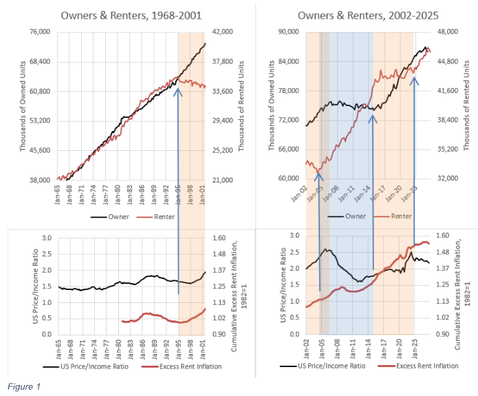
A closer look at 21st-century investment, price, rent, and construction patterns at the aggregate national level confirms the evidence from the 20th century. Figure 1 compares trends in renter-occupied (i.e., investor-owned) and owner-occupied housing in the top panels, and in home price (aggregate price-to-income ratio) and rent (excess rent inflation) in the bottom panels. This includes all types of homes.
1965 to 1995
From 1965 to 1995, the number of both renter and owner households increased proportionately, with little deviation from this trend. Both prices and rents followed flat trends.
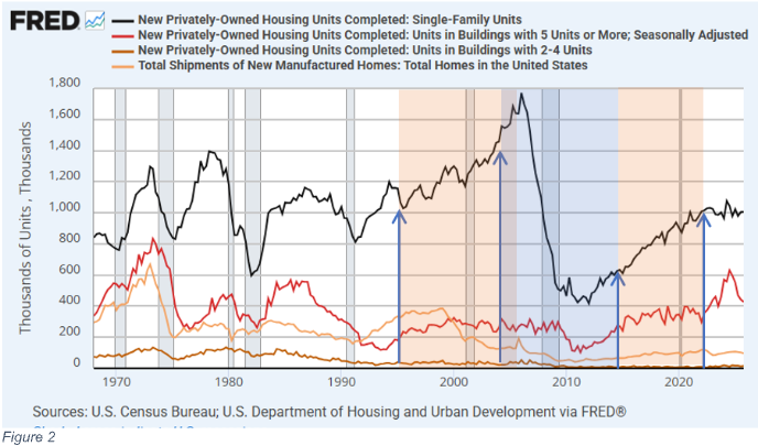
During that period, as shown in Figure 2, the construction of single-family homes fluctuated widely across the business cycle, but the cyclically neutral rate of construction remained relatively stable. The construction of every other home type—apartments, small multi-family buildings, and manufactured homes—declined and became less cyclical. Rental housing increasingly shifted from multi-unit housing types to single-family homes. Throughout the 1980s and early 1990s, the number of new single-family homes outnumbered the number of new homeowner households. Each year, on net, some homeowners moved out of existing homes into new homes, and small investors purchased those existing homes to manage as rentals.
The well-documented expansion of urban land use regulations was an important factor in the decline of multi-family housing types. So, as the 20th century neared its close, choices in the stock of homes were starting to reflect supply constraints across multi-unit home types. But until the late 1990s, the supply of homes wasn’t constrained enough to create competition among renters (and investors) and owners. Household formation continued to rise in proportion to population growth, economic progress, and cultural preferences for both renters and homeowners. Where multi-unit home types were unable to meet demand, investors purchased existing homes to manage as rentals.
Most importantly, for the purposes of the question at hand, the rise of investor activity in the market for existing single-family homes was not inflationary before 1995, even though they were net buyers for much of the late 20th century, because investors never systematically outbid homeowners. They depend on homeowners to be sellers when they increase their positions. Homeowners were selling older homes and moving into new homes, and investors bought those older homes. If homeowners had become net buyers of existing homes in those years, investors would have become sellers.
1995-2004
In the second half of the 1990s, homeowners became net buyers. From the end of 1995 to the end of 2004, excess rent inflation accumulated nationwide to 16% while the aggregate price/income ratio increased from 1.6x to 2.4x. That inflation was associated with an unprecedented decline in renter households (and investors).
During this period, there was a slight uptick in homeowner household growth, but overall, when summing owners and renters, household growth was slower than in the 1970s and 1980s. This highlights two points. (1) As discussed above, funded family homeowners are the primary price setters. When they dominated the market after 1995, prices increased. Higher prices were associated with fewer investors. (2) Rents also increased during that time. If higher prices were the result of more demand from home buyers, that should have led to increased construction and lower rents. Average rents didn’t decline, because urban land-use obstructions were starting to bind. Where cities were unable to grow, rents and prices were now on a permanent upward trend. Where new homes are prevented from meeting local demand, homeowners—housing’s most powerful buyers—bid up the price of the limited supply of homes, and investors sell.
In Figures 1 and 2, the blue arrows and the orange and blue shading indicate where trends in household formation have taken sudden turns. The first turn was a downturn in renter households in 1995.
Expanding credit conditions certainly were a factor in driving up prices and increasing homeownership. But, rising home prices from 1995 to 2004 were not associated with a historically unusual increase in housing demand. Fewer households were formed from 1995 to 2004 than from 1985 to 1994.
Likewise, the significant difference between the 1995 to 2004 period and previous periods of economic expansion was not a higher number of new single-family homes. Rather, there were fewer apartments, multiplexes, and manufactured homes. In 2004, on a per-capita basis, the number of completed single-family homes was similar to cycle peaks in the 1970s, while the number of completed homes of other types was at levels associated with 20th-century recessions.
The unresponsive supply conditions were especially poor in the most expensive urban coastal markets—New York City, Los Angeles, San Francisco, and Boston—which will be referred to collectively as the “closed access” markets. About 5 to 6 new homes needed to be constructed annually per 1,000 residents to accommodate household formation associated with national population growth rates at the time. That amounted to about 1 million units, nationwide, in 1965 and more than 1.5 million units by 2004. Collectively, the closed-access markets have permitted about 2.2 new homes per 1,000 residents annually since 1995. For reference, the Midwest region permitted 5.2 new homes per 1,000 residents from 1995 to 2004 – more than twice the rate of the closed-access cities.
Supply constraints have been especially binding in those markets, and since at least the mid-1990s, the margin that shifts to bring those markets into equilibrium has been outmigration. In a typical year,net domestic migration out of those metropolitan areas numbers in the hundreds of thousands of residents.
From 1995 to 2000, the population of the US outside those cities grew by just under 14 million residents, equating to about 6 million new households. About 1.7 million of those new residents, 12% of the total, were transplants from the closed-access markets.
Those transplants didn’t disperse uniformly. From the West Coast, they moved to inland California, Arizona, and Nevada; from the Northeast, Florida received an unusual share of the outflows. So, rent and price appreciation were very regional in the early 2000s. In the closed-access cities, supply was so binding that normal household formation trends were untenable. The cities generally associated with housing bubbles in Florida, Arizona, and Nevada saw a spike in demand due to outflows from closed-access markets. That demand tested the local capacity and willingness to build new homes at a faster pace. They will be referred to as “contagion” markets.
By 2005, outmigration from Phoenix was rising because the influx of households from Los Angeles had increased the demand for new homes in Phoenix beyond the local market’s ability to increase supply. Local construction capacity was stressed. At the peak of the housing boom, the construction of homes couldn’t keep up with the demand from Los Angeles, and so families had to start moving away from Phoenix, too. The housing supply crisis in Los Angeles spread to Phoenix. The fixation on the credit boom as the cause of rising home prices has led to a conventional wisdom on this period that is wildly misinformed on many margins, such as the idea that Phoenix and Las Vegas filled up with vacant spec homes because overoptimistic builders constructed thousands of homes in locations where they weren’t needed. Those homes were largely sold before construction began to the thousands of families moving out of California. Builders in Arizona in 2005 were holding lotteries to match unstarted homes to new buyers. When migration from California slowed, the builders went from holding lotteries to slowing housing starts sharply in 2005, well before the financial crisis metastasized. Well after that slowdown occurred, the market collapsed when the recession, together with newly tightened mortgage access suddenly, temporarily, stopped the migration flows.
2004-2006
In 2004, renter household formation rose again as suddenly as it had fallen in the 1990s. The subprime lending boom, facilitated by the sudden rise of mortgages funded and securitized outside the federal mortgage agencies, dominated mortgage funding trends from late 2003 to early 2007. Those unconventional new mortgages were utilized by both investors and homeowners. From mid-2004 to mid-2006, household formation briefly returned to the 20th-century pattern wherein both renter households and owner households proportionately rose. Prices spiked where there was competition for limited housing—the closed access markets and the contagion markets—and prices generally remained moderate where housing supply was ample, and an increase in owner households didn’t require a decrease in renters. Typical home prices rose 69% in Phoenix and 5% in Dallas over those 2 years.
Housing trends in most of the country—just about every city between New Jersey and Nevada—were much closer to Dallas than to Phoenix. Construction of new homes was healthy in those regions, but not unusually high, as were home prices. Housing markets were cyclically strong in those areas, but not in any condition that would have been described as a bubble. As noted in the discussion of Figure 2, taking all types of homes into account, new construction was not unusually high. Completed new homes per capita, at the peak in 2006, was lower than it had been in all mid-20th century economic expansions, and year-over-year growth had been unusually muted relative to earlier cycles.
The brief 2-year period from June 2004 to June 2006 was the only time between 1995 and 2022 when both new renter and new owner households were forming. They were forming at about the same rate as had been typical across the 20th century. Yet, those 2 years are associated with the peak of a housing bubble because the closed-access cities were politically unwilling to permit enough new homes to accommodate normal growth rates.
Rents and prices continued to rise during those two years. Across markets, rents were rising more in the closed-access markets where families were being displaced and less in the markets the displaced families were moving to, where more homes were permitted. Cross-sectionally, even during this short period, investors were increasing their market share in ZIP codes with the weakest price trends.
2006-2015
Owner households suddenly stopped growing in 2006 and didn’t start rising again until 2015. New single-family home construction dropped sharply when the growth of homeowner households stopped.
In fact, investor demand appears to have been relatively stable when homeowner demand first declined. Even though the number of multi-family units under construction was much lower than in the mid-20th century, it remained stable for more than two years after single-family home construction collapsed, until the climax of the financial crisis in 2008. But since homeowners are so much more powerful a source of demand for single-family homes, the investor demand that replaced them couldn’t create stability in prices or construction of single-family homes in their absence.
This combination of outcomes is consistent with a market where new multi-family construction was tightly limited by non-market factors like local zoning restrictions, and the prices of new single-family homes were driven by homeowner families at prices generally higher than the price that investors would pay.
Think of the 2006 to 2011 period as a natural experiment highlighting how far small investors were below families with mortgage funding in the 20th century, in terms of marginal price-setting. When homeowner demand collapsed, the aggregate real estate value-to-income ratio declined from 2.6x to 1.7x.
More than 4 million renter households were formed between 2006 and 2011, and another 4 million were formed between 2011 and 2016.
In 2010 and 2011, large institutional investors started making small purchases, and then they increased their activity in 2012. But by 2016, they still only owned about 200,000 units. They surely formed a bottom in some markets where the ability of small-scale investors may have been stretched thin. But 200,000 units isn’t a significant presence in a market of nearly 100 million single-family homes.
While small-scale investors had not produced a floor in home prices when family demand stopped growing, they had been buyers all along. Large investors didn’t enter the market until the price/income level was near its bottom.
2015-2022
In any case, a bottom did form, and when the tug-of-war flipped again in 2015, the aggregate price/income ratio had stabilized at about 1.8x. (The valuation gap from 2006 to 2015 is about where Oosthuizen’s cost estimates, discussed above, would point to.) From 2015 to 2022, renter household formation flattened again, while owner households returned to linear growth. The trends of 1995 to 2004 repeated. Homeowners were buying existing homes from the rental market on net. And, again, rents and prices increased.
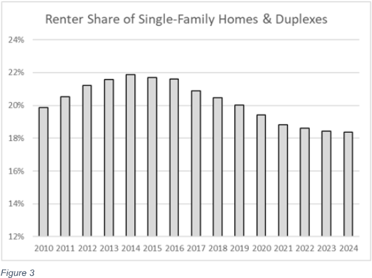
According to the Census Bureau (Figure 3), the share of the stock of single-family homes occupied by renters peaked in 2014 at 22% and has declined every year since. Investors have been net sellers of single-family homes for the past decade as the aggregate price-to-income ratio has risen back above 2x. By 2015, multi-family construction had recovered, so some renter families were able to transition from single-family homes to multi-family homes. But municipalities do not permit multi-family construction to rise enough to offset the crowding out of rented homes from the single-family housing stock. So the increase in homeowner households since 2015 has driven high, regressive rent inflation as renters lose units.
2022-Present
Since 2022, however, the portion of single-family homes used as rentals has started to stabilize. And, looking back at Figure 1, this is because the housing market has returned to the 20th-century norm. Since 2022, renter and owner households have increased in proportion.
This has coincided with a reprieve in rising rents and prices. Looking back at Figure 2, this period was associated with a temporary spike in apartment construction. From the end of 2022 to the end of 2025, 1.7 million renter households formed, and 1.5 million apartments were completed. So, about 200,000 renters have moved into single-family homes, on net. That equates to some positive growth, but to a declining share of single-family units occupied by renters (owned by investors). And, though it was even more of a lagging development than the entry of large-scale investors in the existing home market had been, there is now a growing market of new single-family homes purposely built as rentals. More than 200,000 new single-family rentals were completed over that time, so home buyers are still marginally crowding out renters (investors) from the existing-home stock.
Apartments take, on average, nearly 2 years to build after the ground is broken. After the brief increase in completions, apartment starts declined to below 400,000 in 2024 and 2025, so if demand for renter household formation continues to grow, it will require more single-family investors.
Notes on Supply and Demand
Whether any home buyer affects the local market productively by increasing the supply of homes or unproductively by driving up the rent or price of homes is a product of supply conditions.
Figure 4 notes the effect new buyer activity should have on home prices and rents. Where new homes cannot be built, and more buyers cannot increase the number of homes, prices increase. Where new homes can be built, buyer activity will raise existing home prices above the cost of constructing new homes, triggering new construction, which keeps home prices near the cost of constructing new homes on marginal lots at the edge of the metropolitan area.
Thus, where new homes can be built, additional investor interest in buying properties should lead to lower rents. One could think of this in simple price and quantity terms—more homes will lower rents, all else equal. Or one could state this in yield terms. If investor demand increases, meaning that they decide to accept a lower return on investment, new buildings will keep prices level while rents decline.
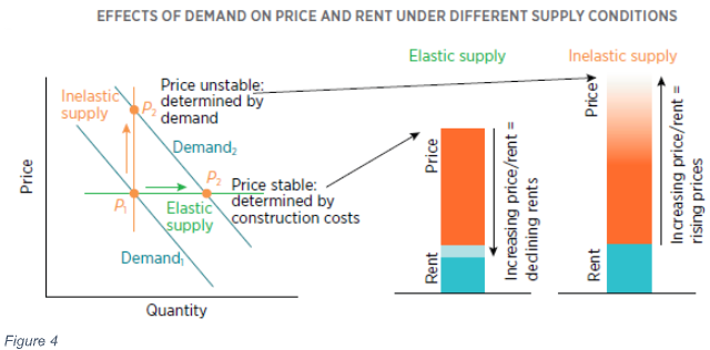
Figure 5 visualizes how this process has unfolded nationally since 2005. Funded families are generally willing to pay more for homes than investors are. They accept lower yields on the rental value of their homes because ownership itself has value. So, when buyer demand stopped growing after 2005, home prices across the country declined, as the investor market had to expand to fill the gap. Prices declined until new investors were attracted to the market.
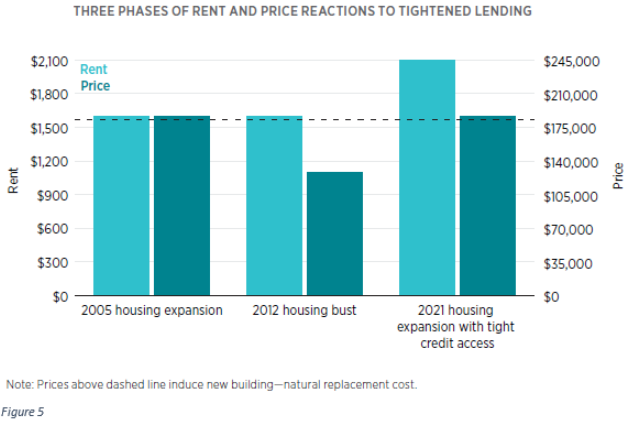
When the shock ended a decade later, home prices were generally well below the cost of new construction. One way of thinking of the aftermath of the pause in owner household formation is that where builders cannot justify paying a positive sum for land, they cannot build new homes. New homes cannot be constructed on land with negative value.
However, existing homes are bundled with land. Land under existing homes can attain a negative value. And, after 2008, many homes in the United States were, effectively, $250,000 properties that were a bundle of a $300,000 home on a lot worth negative $50,000. If there are homes in a city that sell for $250,000, but that would cost $300,000 to build, there is no way for builders to compete with home sellers.
For this reason, the construction of entry-level single-family homes essentially ended after 2008. More than 500,000 new single-family homes had been sold annually at prices below $250,000 before the Great Recession. Eventually, when owner household formation started growing again, both rents and prices increased. In short, in Figure 1, first prices declined, but rents remained relatively flat (as in the middle of Figure 5); then both rents and prices increased (as on the right side of Figure 5). That is a signal that supply was inelastic, as shown in Figure 4. Rising prices only had a weak effect on new construction.
This can lead to spurious conclusions on the topic at hand. This can make it look like the rise of investors caused rents or prices to rise, when changing supply conditions were the cause. The lack of market power held by investors led to lower prices after 2006. Lower prices led to years of reduced construction. And that eventually led to rising rents. The inaccurate presumption that investors have more market power than families has led to confusion about the cause of rising prices and rents.
In Figure 6, when the supply curve (red) is vertical, that means new homes cannot be built and more demand will raise prices. Where the supply curve is flat, it means that new homes can be built, and the new supply will keep prices moderate.
Supply elasticity is not linear, and we can infer this from basic historical trends. The left end of the supply curve is vertical because homes are durable. They don’t go away if demand declines. Demand 1 in Figure 6 reflects the post-2006 period. Supply conditions were similar to the middle bars in Figure 5. Marginally rising prices didn’t lead to more construction because many existing homes were still cheaper than it would have cost to build equivalent new homes.
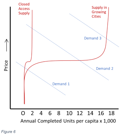
We can infer that there is a broad, flat range where supply is highly elastic because, until the end of the 20th century, homes across the country remained relatively affordable, and rent inflation tracked general inflation. Also, over the long term, there was little difference in home price trends between moderately growing cities and fast-growing cities. Demand line 2 reflects the 20th-century market.
Before 2008, the only markets that deviated far from national home price norms were markets where very few homes were built. In some rust-belt cities, that was because demand was near the left end of the supply curve, and homes were unusually cheap. In the closed-access cities, that was because the right side of the supply curve turned vertical at very low demand levels, and they were unusually expensive.
Since owner-occupied households started growing again, putting upward pressure on prices, housing supply nationally appears to have become inelastic. Many markets now appear to be pinned on the right end of the curve. Prices have increased without triggering much new construction. In many markets, inflationary trends didn’t stop at the right bars of Figure 5. Rents appear to have continued rising, even as home prices have risen enough to justify high land prices in many markets.
Litigating the causes of inelastic supply over the past decade is beyond the scope of this paper, but in addition to high land prices, we can infer that supply has been inelastic in recent years from homebuilder activity. Since 2021, finished new homes have sold more quickly than they had in any previous year in the decades that the Census Bureau has tracked it. Builders have been selling completed new homes as fast as they could complete them. Yet, at the same time, they have been taking longer to finish homes than ever before. There has been no reason for them to slow construction. The last thing a builder wants is half-finished inventory sitting on lots. They couldn’t complete them faster because they struggled to get materials delivered in a timely manner. On both measures, conditions are improving but are not back to pre-COVID norms. Finished homes are selling very quickly, yet builders are struggling to complete homes under construction. That’s a strong signal of supply constraints.
It may seem implausible that the entire country is pinned to the right side of the supply curve. There are many empty places where no new homes are needed. But, where new homes would be filled with families, they must compete for inputs. For example, electrical transformers required to complete the electrical infrastructure and open a new neighborhood have been in short supply since the onset of COVID and continue to face delays measured in years. This leads to inter-regional competition for supplies. Cincinnati can be at the right, vertical end of the supply curve, even if local construction is still relatively low and developable land is available, because inputs like electrical transformers are being diverted to, say, Atlanta, where demand is higher, and the new homes can fetch higher prices. Both markets face limited supply capacity under those conditions.
When investor market share was increasing, American housing was pinned to the left end of the supply curve. When homeowner demand returned, housing eventually was pinned to the right end of the supply curve.
Another question, preliminary to drawing conclusions about the effect of investor activity on housing markets, is: “When has demand been in positions 1, 2, or 3, and why?” And that question has a much more informative answer than the answer to the question, “What effect do investors have on housing markets, using supply elasticities estimated from published models based on local conditions?” The shared changes in supply conditions over the last 20 years have been much more important than differences in local conditions. In the example above, where there is regional competition for shared inputs like electrical transformers, the supply elasticity for each metropolitan area, estimated in, say, a 1995 study, conveys little information about housing supply conditions across the country since 2008. Some of the existing literature on post-2008 housing markets simply makes no account of the deep tightening of credit access that both caused prices to collapse and led investors to fill the gap left by missing homeowners. Authors of those studies have either concluded that local supply conditions don’t matter or that supply conditions have become similarly worse across markets.
Local supply responses since 2008 have been overwhelmingly the result of shared shocks—either the shock of reduced mortgage access that made existing homes too cheap to induce more building or the long, difficult process of reattaining the capacity to produce all the inputs (such as the electrical transformers mentioned above) required to open new neighborhoods. One intention of this paper is to lay out the importance of these shared national supply conditions so that future researchers consider controlling for these changes to avoid reaching specious conclusions.
For example, single-family completions per capita across the entire Midwest Census region have remained permanently below half of the 2006 construction rate, when owner-household growth paused, despite rents and prices for new homes outpacing general inflation by 20%. Why is the Midwest pinned to the right side of the supply curve (meaning that marginal new demand leads to higher rents and prices rather than more construction) at less than half their previous construction rate? Homeowners have been buying homes back from investors, but not enough to elevate home prices to a level that can motivate homebuilders to direct limited inputs to the Midwest instead of to faster growing, pricier markets.
The elevated rent inflation that has occurred across the country since 2015 has not been driven by investors’ market power. It has been caused by their lack of market power. Investors were unwilling to pay for homes at the prices that had generally prevailed when there had been more family buyers because they required a higher gross yield on investment than family buyers do. Rents increased when investor market share was higher after 2015 because homebuilders were uninterested in selling investors new homes at the given rent and price levels. If investors had market power in the homeowner market, they would have been purchasing more new homes from homebuilders, and those new homes would have caused rents to decline. The only way to prevent investor market power from lowering rents is to block the construction of new homes.
Why did owner households stop forming?
The initial cooling in housing markets before 2008 began with reduced buying activity in high-tier neighborhoods of the most expensive markets. Increasingly, though, the decline in owner purchase activity after 2006 was associated with a decline in mortgage funding.
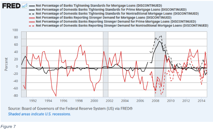
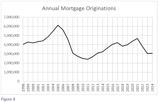
The Federal Reserve’s Senior Loan Officer Opinion Survey on Bank Lending Practices reflects that cooling sentiment. Even by 2004 and 2005, banks reported declining demand for mortgages (shown in red in Figure 7). As Figure 8 notes, mortgage originations for purchases had already declined by 2007. Tightened standards (black in Figure 7) eventually followed after years of declining loan demand, and by 2008, limited access to mortgages was the binding constraint on owner-occupied household growth.
Data from the New York Federal Reserve in Figure 9 confirms that the tightened standards had a practical effect on mortgage originations. This is data for both refinancing and purchase mortgages, so there are spikes in originations in 2003, 2012, and 2020, coinciding with declining interest rates. In both the late 1990s and the years leading up to the 2008 crisis, about 2/3 of originated mortgages, by value, went to borrowers with scores under 760. Over the course of 2008, the proportion dropped to about 40% and has never recovered.
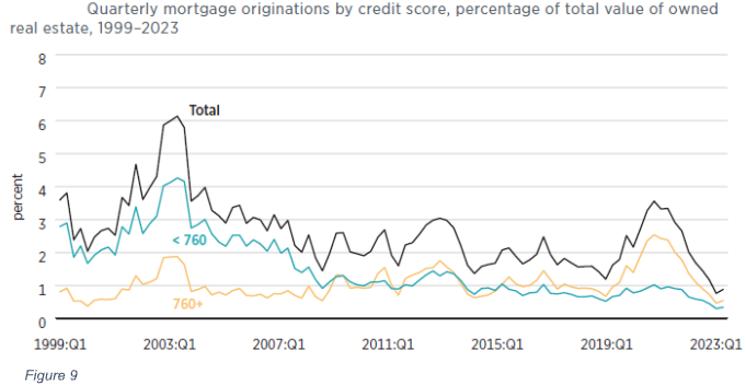
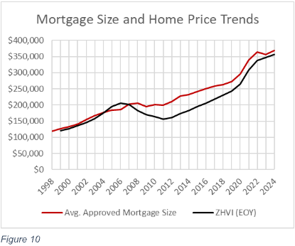
Figure 10 provides other evidence of the shift in lending patterns. Zillow’s estimate of the median US home price, in black, and the average size of originated mortgages reported in Home Mortgage Disclosure Act (HMDA) data, in red, moved in parallel from 1999 to 2007. From the 2006 peak to the 2011 trough, the typical American home lost 24% of its value, but the average mortgage size actually increased over that time. More expensive neighborhoods retained access to mortgages, and less expensive neighborhoods lost it. And, they didn’t just lose access to reckless loan types associated with the subprime boom. Standards permanently changed relative to late-20th-century norms.
These patterns are confirmed in annual SEC filings from Fannie Mae and Freddie Mac. They report average mortgage size and down payments for both new mortgages and for mortgages originated in earlier years. At Fannie Mae, the average credit score on originated mortgages fluctuated around 710 points across both new mortgages and the book of business originated in previous years. By 2009, it had risen above 740 on new mortgages, where it has remained. In 2006, the average value of homes in both Fannie Mae’s book of business and among its newly originated mortgages were about $250,000. Home prices had risen in those years, but Fannie Mae was originating mortgages to the same borrowers in the same homes that they had been for years, if not decades. By 2009, the average price of homes of borrowers paying down Fannie Mae mortgages from previous years had declined to $204,000. The average price of homes getting financed with new mortgages was $327,000. In other words, quite suddenly, the average home Fannie Mae was willing to underwrite and approve a mortgage for was worth 60% more than the average home it had previously been willing to approve a mortgage for, across all homes from previous years and decades that were still paying off their principal.
Of course, the debate over what standards are appropriate in the US mortgage market remains unresolved, but what should not be up for debate is that post-2008 standards have been much tighter than they were for decades before. The standards did not simply reverse subprime excesses. They reversed long-term norms and are largely responsible for the cessation of net new owner household formation for a decade.
Which Households Haven’t Formed
As discussed above, the closed access markets perennially permit too few new homes to accommodate natural household formation—less than 3 units per thousand residents, annually—and so perennial outmigration is necessary for their current residents to form new households. From 2008 to 2012, fewer than 3 units per 1,000 residents were constructed each year nationally. There were few cities with ample new housing to migrate to. So, household formation stalled in other ways. Primarily, young adults remained in their parents’ homes longer.
Among family households, which have at least two related members such as spouses, siblings, or parents and children, the number of adults per household declined linearly from 2.31 in the early 1950s to 2.18 in the mid-2000s, as shown in Figure 11. Then, coinciding with the pause of owner household growth and the collapse of new home construction, the trend immediately reversed. Today, there are as many adults in the average family household as there were in 1951.
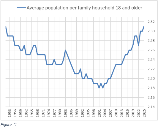
Compared to the pre-2006 trend, there are 14 million extra adults living in family households. If they had followed the pre-2006 trend in household formation, they would have formed 10 million new households. (Some of them would have taken on roommates or married.) Those new households would have mostly been renters, especially with the new mortgage standards.
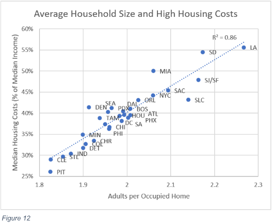
Figure 12 highlights that the stress of inadequate supply affects household size across space as well as across time. In cities with higher housing costs, households are predictably larger. Before 2008, housing supply was regionally constrained, and since then, it has become relatively universally constrained.
The slowdown in household formation creates a bias in homeownership measures. The blue line in Figure 13 is the reported national homeownership rate. The homeownership rate is a ratio of households—the number of owner households divided by the number of total households. The red line shows what the homeownership rate would be if adults had continued moving out of their parents’ homes following the trend dating to 1951.
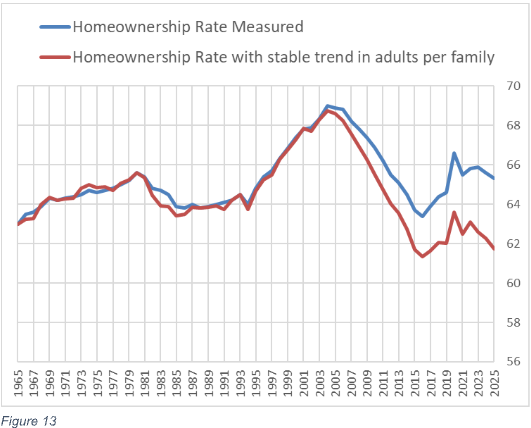
The red line more accurately portrays the effect of the 2008 crackdown on mortgage access. Fewer adults are able to access mortgage funding to buy homes today compared to the period from 1965 to 2007, so the homeownership rate has settled at a lower level—about 62% if we treat adult children living with parents as “would-be households”. The difference between the homeownership rate in 2006 and today is about 10 million households that were owners or would have been owners but are not today. In Figure 1, those equate to the roughly 10 million households that flattened the owner trend and raised the renter trend from 2006 to 2015.
If the adults still living with family form 10 million households, under current lending conditions, it will be associated with a declining homeownership rate. Of those 10 million households, less than 2 million would be owners if they followed the pre-2008 trend. The other 8 million would be renters. The trend in household formation since 2022 offers a glimpse of what that would look like. The number of owner households has continued to rise, and owner households have continued to poach rental homes from the existing stock of single-family homes, but the homeownership rate has declined. That was associated with a brief rise in the number of apartments that were completed. Until local land-use reforms begin to allow more multi-unit construction, marginal growth in new homes will need to be in single-family homes, and unless post-2007 changes to mortgage access are radically reversed, the households that will form as those homes are constructed will be mostly renter households. They will be households that need investors.
Figure 13 actually understates current access to mortgage funding compared to the 20th century, because of baby boomer demographics. Older households have higher homeownership rates than younger households under any market conditions, and the average age of American households has increased substantially over the last 60 years. The homeownership rate within age groups was about the same in 2004 as it had been in 1982.
Are investors crowding families out of housing? No, homeowners are crowding out investors (and renters). Figure 14 shows the percentage of all residential real estate by market value. The portion of residential real estate, by value, that is owner-occupied is at a record high.
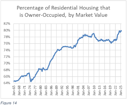
How can that be, when the homeownership rate has declined? First, it’s because of those 14 million adults living with their parents. Those homes are “owner-occupied” even though they are housing millions of adults who would be renters if there were more investor-owned homes. Another reason is that families that still have access to mortgage financing have continued to buy and consume housing similar to what they would have lived in before 2008. But renters who have been subjected to regressive, high rent inflation have been curtailing their housing consumption for budgetary reasons.
Or, to describe it from another angle, the renter families who had to move out of the 4% of the single-family stock when owner households purchased those homes over the past decade (Figure 3) moved into apartments, which tend to be less valuable than single-family homes.
There are likely nearly 10 million would-be renters waiting for investor-owned homes that will allow them to form new households. Many of those will need to be single-family homes, under current regulatory conditions. Many of them will likely need to be purpose-built single-family rental homes, as owner-occupied households are still buying existing rentals. And, at the scale they are needed, they will likely require some deep-pocketed investors.
Asking the Wrong Questions
“The Influence of Institutional Single-Family Investors on Homeownership: Who Gets Targeted and Pushed Out of the Local Market?” by Brian Y. An, Assistant Professor at the School of Public Policy and School of City and Regional Planning at Georgia Institute of Technology, takes a common approach of blaming investors for crowding families out of the market. Even though An mentions, in passing, the effect of tighter mortgage access as a constraint on buyers, he centers large investors as the causal agent behind lower homeownership in the Atlanta region.
He refers to investor activity as “home equity theft.” Where large investors purchase more properties in neighborhoods with high minority representation or lower socio-economic characteristics, he refers to their activity as “systemic targeting”. He finds that “if a census tract neighborhood experiences from zero market activity of corporate investors to a fully concentrated corporate investment in the single-family housing market, its homeownership decreases by 3.6% down. In terms of its average effect size, it translates to a 1.3% decrease throughout the ten-year period, explaining about 25% of the single-family homeownership decline among the Atlanta metro neighborhoods during 2007-2016. Hence, the effect size is seemingly quite substantial.”
Figure 15 and Figure 16 are from An’s paper. Figure 15 shows that the homeownership rate in Atlanta declined sharply from 2007 to 2013, then flattened out.
Figure 16 shows that large institutional buying activity was practically non-existent until 2012, then rose sharply in 2013 and 2014, before declining sharply from the peak.
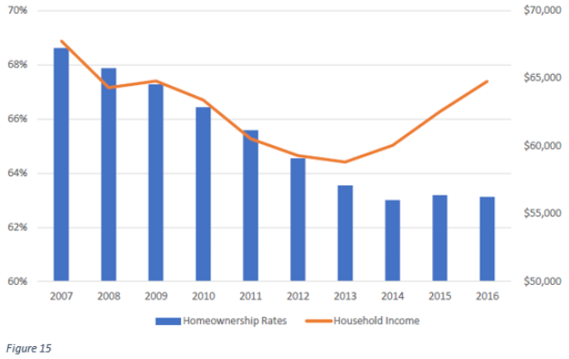
An finds that neighborhoods “targeted” by large investors saw much larger declines in homeownership rates than neighborhoods not “targeted” by them. He finds that medium and small investors did not have the same effect.
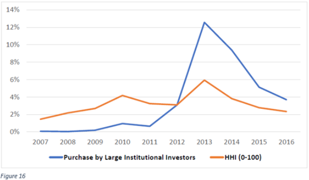
But, more than 90% of the decline in homeownership in those neighborhoods happened between 2007 and 2013. The more likely explanation for these findings is that large institutions are the last movers in these markets. A tremendous amount of capital from medium- and small-sized investors flowed into real estate markets after 2007 amid an economic meltdown. When it reached its functional limit, prices continued to fall in neighborhoods with no buyers. Finally, large investors filled that chasm. Where more families were now locked out of mortgage markets, eventually more large investors were required to help those neighborhoods find a bottom.
Atlanta single-family housing markets historically had cleared through the construction of new homes to meet household formation demand. Throughout the period when homeownership was declining, new construction was collapsing. Today, new single-family construction in Atlanta remains at half its pre-Great Recession levels.
If investors are crowding out families, why aren’t homebuilders constructing more homes for families that want to buy them? This was always the way new households distributed themselves into homes in Atlanta. Of course, it was always the way that households distributed themselves into homes. When families demand more homes, new homes must be built.
Meanwhile, while the mortgage crackdown suppressed single-family construction, multi-family construction was not able to fill the gap. Atlanta, along with almost all major American cities, uses strict zoning rules and other obstructions to make building multi-family homes very difficult.
Clearly, when large investors started buying homes in Atlanta, home prices were too low to trigger normal market activity, such as new construction. Clearly, households were not being priced out of homes (Figure 17).
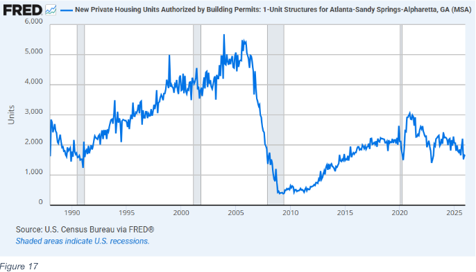
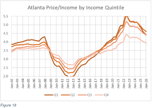
Figure 18 shows the price/income trend of ZIP codes in Atlanta from 2002 to 2026. Before the Great Recession, price/income ratios from about 3.5x to 4x were associated with valuations that could trigger new home construction for new households.
Between 2007 and 2012, in ZIP codes with above-median incomes, price/income ratios dropped from 3.6x to 2.6x. In the lowest-income quintile, the typical price-to-income ratio dropped from about 4x to about 2x. The brief spike in large institutional buying activity from 2013 to 2015 was associated with a recovery in prices back to a level near the 2010 lows, but that was still far too low to create a functional market where new homes could compete with the deflated prices of existing homes so that construction could recover to pre-recession levels. The mortgage crackdown was so overwhelming that, after it happened, the poorest residents of Atlanta could have bought the homes they were living in with fewer years’ of income than the richest residents of Atlanta could have.
Capital was flowing into a market that desperately needed it. An finds that large institutional buyers were cross-sectionally associated with declining homeownership. Those sellers were not being crowded out. Families selling during those years at deep discounts were selling under duress due to financial stress in a market where they had frequently lost all the equity in their homes. The “theft” of home equity wealth occurred from 2007 to 2012 and ended when large investors provided a floor.
In a review of investor activity in the Charlotte region, Sean Kodama Brunson found that “On average and at various points on the sale price distribution, all types of investors pay a discount relative to owner-occupiers. This discount is both statistically and economically significant.” He found that prices tended to increase slightly after investor buying activity. “Since 2012, home prices in the Charlotte region have increased about 5.61%-5.75% per year. However, the results… suggest that an increase in investor activity only increased home prices by about 0.32%-0.59%.” Finally, he notes, “Regardless of race or income of the individuals in a given area, institutional investors did not outbid owner-occupiers.”
One source of confusion on this topic is that national home value indexes appeared to simply revert to normal around 2012. In Figure 1, the national aggregate price/income ratio in 2012 was similar to the long-standing 20th-century norm. This creates a temptation to benchmark against markets around that time, and since 2012 is when institutional investors began building their portfolios, it seems like the natural point at which to test their effects on the market.
But not only are these the wrong questions, the benchmark is also perfectly aligned to provide the wrong answers to them. The majority of the elevated aggregate real estate value before 2008 stemmed from the deeply undersupplied closed-access markets. Homes lost value in the closed-access markets after 2007, but they were still inflated relative to 20th-century norms. In most of the rest of the country, as in Atlanta, home prices had never been particularly elevated, and by 2012, in neighborhoods that were sensitive to credit conditions, they were deeply discounted.
Home prices in the poorest ZIP codes in Atlanta inevitably would rise after 2012 because they were far too cheap to spur enough new construction to meet the natural demand for household formation. Prices bottomed in 2012 because large-scale investors entered markets where other capital had failed to create a price floor. Their presence in ZIP codes where prices subsequently recovered back to equilibrium levels creates a spurious correlation between investors and price trends. Benchmarking prices and investor activity to 2012, when they established their footprints, is analysis optimized for identifying spurious correlations.
The change in mortgage access in 2008 led to a decline in home prices that was correlated with local incomes and sensitivity to credit access within each market. On the question of whether investors came to the market or the market came to investors, Figure 18 leaves little doubt. Our overwhelming presumption should be that collapsing prices moved the market for home purchases to investors. Where home prices were at half their historically normal levels, there is little reason to suspect that changes in investor demand drove the shift toward investor activity. Investor sentiment and activity were driven by collapsing prices. If homes in growing cities had been selling at half the price it would cost to replace them in 1990, 1995, or 2000, investors would have similarly increased their ownership.
Investors Across Markets
This pattern isn’t unique to Atlanta. It happened across markets. Homeowners went missing. Prices collapsed. Investor capital was stretched thin. Eventually institutional investors helped create a floor.
Figure 19 compares cumulative home price trends in 98 metropolitan areas from 2005 to 2026. They are sorted into quintiles according to how much investor market share of single-family homes grew from 2004 to 2012. The average investor market share of single-family homes in the first quintile (blue) was 4.6% in 2004 and increased to 5.5% by 2012. The average investor market share of single-family homes in the fifth quintile (black) rose from 12.2% to 21.7%. Over a period of 8 years, investor capital had to find its way in to nearly 10% of the entire stock of homes in those markets. Clearly, collecting and directing that much capital into a new sector is a tall order.
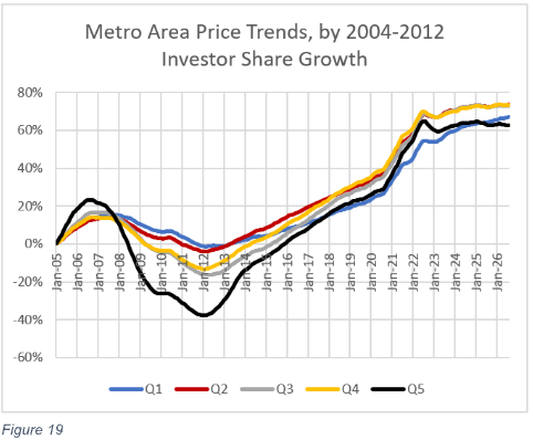
The more investor capital was needed, the more prices collapsed while that capital found its way to the real estate market. Overwhelmingly, over time, across cities, within cities, however you cut it, investor market share trends have been negatively correlated with home price trends.
Then, after 2012, prices across those markets reconverged back toward similar cumulative trends. While that happened, investor market share declined as homeowners started outbidding investors again. And, the trends again held cross-sectionally. In the metropolitan areas in the first quintile, investor market share actually continued to rise moderately. In the fifth quintile of metropolitan areas, investor market share fell from 21.7% back down to 15.5% by 2026 as prices reconverged toward cumulative trends similar to other markets.
More Important Questions
The effect investors have on the local market depends on whether new homes can be built. The key question regarding the economic condition of families is: “Why are prices going up instead of the quantity of homes?”
Before 2008, the key constraint was zoning. Zoning limited the total number of homes in closed-access cities and the number of multi-unit homes in most other cities. The literature on this problem is accumulating. A century ago, in 1926, the Supreme Court ruled in Village of Euclid v. Ambler Realty Co. that cities could create zones that separated nuisances from residential areas. In this case, the nuisance was apartments. Over the following century, cities increasingly imposed legal limits on the construction of apartments.
Frequently, the limitations were implicitly or explicitly racist and classist. Atlanta originally had “White Districts” and “Colored Districts.” When the courts ruled them unconstitutional, Atlanta relabeled the “White Districts” as single-family-only zones and the “Colored Districts” as “Dwelling House Districts,” where apartments could be built.
On the margin, renters and investors have some oppositional interests. Renters would prefer to pay less, and investors would prefer to charge more. Renters would prefer lenient eviction standards (for themselves, if not for their disruptive neighbors) while investors would prefer to more easily remove residents that are disruptive or non-paying. But, much more importantly, renter households and investors have a symbiotic relationship. One can’t exist without the other.
Given the racial and class history aimed at corralling or excluding renter families, we should not neglect that symbiosis. One could describe opposition to investors in single-family housing as the last in a long line of efforts by municipalities to exclude families of lower socioeconomic status: first, in the 20th century through the limitations on apartment building; then in 2008 through the tightening of mortgage access that families used to buy entry-level single-family homes; and now finally with laws to obstruct investors in single-family homes so that renters are excluded from those neighborhoods, too.
From 2007 to 2015, the homeownership rate for white families declined from 75% to 72%. The homeownership rate for black families declined more steeply, from 48% to 42%. Some of the existing literature seeks to blame investors for the decline in homeownership. If investors are instead simply filling the gap left when other factors caused homeownership to decline, that literature, whether deliberately or inadvertently, supports the continuation of some of the darkest currents in American policymaking. This warrants a “first, do no harm” approach when considering new policies that aim to remove any willing participants from the housing marketplace.
Yale Law professor David Schleicher has documented how the accumulation of zoning laws has muted the ability of American families to move to cities that would otherwise have the potential to grow but cannot because of binding, arbitrary land-use rules. Schleicher focuses on muted mobility, such as families who remain in regions that lack economic opportunities because housing in the zoned urban areas is too expensive, but as zoning has limited the growth potential of cities, it increasingly induces involuntary mobility. The closed-access cities have very high perennial net domestic outmigration. That has become their primary source of housing for new households, either from local population growth or newcomers. From 2010 to 2020, the Los Angeles metropolitan area permitted about 270,000 new homes. During that same period, about 420,000 more families moved away from Los Angeles than moved into Los Angeles from other parts of the country. For every two new homes built during that period in Los Angeles, three newly vacant homes were created by the regional displacement of former residents.
Many of the remaining families in Los Angeles are living with financial stresses and dilemmas similar to those of families in poor regions. There are important personal reasons that tie them to a location where they will be poor. For families in poor regions, those connections and frictions to economically advantageous migration are easy to see. In cities like Los Angeles, the effect is more subtle because the poverty is caused by high rents.
Zoning initially limited opportunities to move to new places. But now that some metropolitan areas have entirely lost the ability and willingness to grow, the problem has moved to a new, worse regime. Now, displacement is required. Many families face the dilemma of moving away from a neighborhood or an entire region where they have important personal connections. The population of the Los Angeles metropolitan area peaked in 2017 and has been declining since. In a city like Los Angeles, rents must systematically rise each year high enough above the previous year to induce more families to choose displacement.
In many cases, rising rents are eating up all of the growth in family incomes. Despite higher gross incomes than in other regions, incomes after rent in the closed-access cities are lower, especially for families with below-average incomes. Since 2008, the depressing effect of rising rents on the finances of families with below-average incomes has spread to other cities.
In this context, asking whether there are too many real estate investors or whether they hurt local housing economics is a deeply misguided question. If investors had been able to purchase more homes in the years after 2008, millions of American construction workers would have remained employed, and rents on homes in cities across the country would be much lower today. In cases where local land use rules produce regional displacement, at least other markets could have presented the displaced families with new homes rather than rent inflation.
Analysis of trends in home prices, rents, and investor activity
In a new paper I have co-authored with John Welborn from Dartmouth College and Drew Lehe, we review additional literature on the effects of investor capital. We attempted to more fully identify the causes of the decline in home prices after 2007 and to examine how investors and homeowners have interacted since then.
We analyze and discuss several important points:
- Tightening lending standards was the most important factor associated with declines in home prices and homeownership.
- The capital of small real estate investors was stretched thin. In ZIP codes hardest hit by the mortgage crackdown, a more than 50% price decline was associated with only an increase of about 1% in investor market share. If more investor capital had been available, prices would have been much more stable.
- Eventually, rising prices were highly correlated with a reversal of the price collapse. Where collapsing prices had created a shock to local new home construction activity, rents and prices had to increase for construction to return. The supply shocks tend to create more rent inflation in poorer neighborhoods, because families in those neighborhoods have fewer resources to bid for the inadequate supply of homes as new households with more resources form. Investor activity was not highly correlated with rising prices. In fact, they were correlated with lower prices after accounting for the other factors.
How could that be? Surely, any source of demand will raise prices. How could more investors be associated with lower prices? The answer lies in motives. And the trick to understanding statistical analysis of housing during this period is to recognize that, with a fixed supply of homes in a given neighborhood, rising investor market share can result from declining demand from homeowners or rising demand from investors. Prices provide an easy answer to that question. Where rising investor market share is associated with rising prices, then we can infer that investors have decided to buy more homes in that neighborhood, all else equal. When rising investor market share is associated with falling prices, we can infer that investors are replacing homeowners who have lost the ability or willingness to buy homes in that neighborhood.
In causality tests, we found that before 2012, when home prices were generally declining, investors were investing in ZIP codes that had declined deeply in value. Prices declined less after the investors arrived than they had before they arrived. They couldn’t entirely replace the exodus of homeowners. Where homeownership was declining sharply, prices were declining, but less so than if investors hadn’t been active. Where homeownership was rising, investors were more willing to sell properties to the new homeowners, so that the new demand from homeowners didn’t cause prices to increase as much as they would have without investors.
But what we found after 2012, when prices across the country started to recover, surprised us. Where homeowners were purchasing more homes, prices tended to decline, and where homeowners were more likely to be sellers, prices tended to rise. This can’t be explained by investors who are merely price sensitive. This requires investors who are choosing to exit markets where homeowners want to buy and enter markets where homeowners want to sell.
This is highly unusual. For a variety of reasons, ZIP codes with rising demand should see demand increase across all types of buyers. One way to explain this is that investors and homeowners have different motives. Homeowners want to live in neighborhoods that match their preferences. As noted above, willing and able homeowners generally outbid investors. When homeowners are buyers, home prices rise relative to their rental values. Investors want to earn a return on their investment. They purchase homes whose prices are low relative to their rental values.
Investor demand was negatively correlated with homeowner demand because the rise in investor market share was driven by the decline in homeownership. And the decline had been so sharp that by 2012, many neighborhoods needed more investor capital, even though home prices were well below the level investors would consider attractive under normal circumstances.
As markets slowly normalized, neighborhoods where homeowners could still qualify for mortgages returned to pre-crisis prices more quickly. And, when they did, investors lost interest. They could earn better returns by selling those homes and reinvesting in neighborhoods where potential homeowners were still struggling to obtain mortgage financing in other markets. Eventually investors started purchasing new homes in some markets as homeowners bought up existing homes.
Investors were selling out of neighborhoods where families could purchase homes, and buying homes in neighborhoods where federal regulators tightly control whether families can purchase homes.
The shift among small investors from being associated with slower price inflation when families are buying to being associated with relative price deflation where families are buying has as much to do with the homes they are selling as with the homes they are buying. They have been net sellers since 2014. A lot of their activity is associated with the wide array of outcomes related to when they bought their properties and where, whether they suffered through some losses before markets turned around, etc.
Large investors, while they still own an exceedingly small portion of single-family homes, didn’t start purchasing homes until about 2012, at the market bottom. And, when they did, they were especially keen to purchase in the deeply discounted markets. They have generally remained buyers; they have continued to favor discounted markets; and they have been learning to be more efficient and lower their cost of managing properties. Unfortunately, this makes them vulnerable to motivated reasoning by those for whom they are presumptively the “bad guys.”
Conclusion
In the face of these developments, there is now a running debate about whether to prevent investors from purchasing more homes. This would be exceedingly harmful to the millions of Americans that have delayed forming new households since 2008. Renters need investors. And, however you slice it, growth of investors has always been associated with moderation in housing costs. There is no sense, in the aggregate, in which investors are pricing out potential homeowners. The truth is closer to the opposite. Investors, in the aggregate, don’t set higher market prices than homeowners do. And what potential renter households desperately need is a housing market that welcomes investors, rather than one where homeowners have crowded them out.
Endnotes
- See Figure 1 for sources of residential real estate value. Estimate of residential investment is from the Bureau of Economic Analysis. The estimate is Net Residential Investment from Table 5.2.6. Real Gross and Net Domestic Investment by Major Type, Chained dollars.
- Cortright, Joe. 2016. “The Illegal City of Somerville.” City Observatory, June 15. https://cityobservatory.org/the-illegal-city-of-somerville/.
- Mich, Luke Anthony. 2017. “The Missing Middle: Understanding Low-Rise, Moderate-Density Housing in Greater Boston.” Master’s thesis, Massachusetts Institute of Technology. https://dspace.mit.edu/handle/1721.1/111424.
- U.S. Census Bureau, “TENURE BY UNITS IN STRUCTURE,” American Community Survey 5-Year Estimates Subject Tables, Table B25032, 2010, https://data.census.gov/table/ACSDT1Y2024.B25032
- Lee, Keyoung and Wylie, David, Institutional Investors, Rents, and Neighborhood Change in the Single Family Residential Market (July, 2024). FRB of Philadelphia Working Paper No. 24-13, Figure 1 Available at SSRN: https://ssrn.com/abstract=4890473 or http://dx.doi.org/10.21799/frbp.wp.2024.13
- Chris Nebenzahl, Rick Palacios Jr, Danielle Nguyen, and John Burns, “The housing bill that will make affordability worse, not better”, John Burns Research and Consulting, March 6, 2026. https://jbrec.com/insights/21st-century-road-to-housing-act-impact/
- A review of some of the literature will follow, but it will require some preliminary discussion.
- 21st Century ROAD to Housing Act, Section 901, https://www.banking.senate.gov/imo/media/doc/section_by_section_final.pdf
- Michigan House Bill 6074 and Oregon House Bill 4128
- Census Bureau New Residential Construction, Quarterly Starts and Completions by Purpose and Design. https://www.census.gov/construction/nrc/data.html
- See US Government Accountability Office, “Rental Housing: Information on Institutional Investment in Single-Family Homes” GAO-24-106643 Published: May 22, 2024. Publicly Released: May 22, 2024. https://www.gao.gov/products/gao-24-106643
- Oosthuizen, D. (2023). Institutional Housing Investors and the Great Recession (Working Paper No. 23-22). Federal Reserve Bank of Philadelphia. https://doi.org/10.21799/frbp.wp.2023.22
- Oosthuizen, Page 13, Table 1, Column 5. Specification in columns 1 through 4 have slightly different estimates, but in all cases, the rank of the 3 owner groups is the same.
- Household counts are from Table 8 (Quarterly Estimates of the Housing Inventory: 1965 to Present) of the Census Bureau’s Housing Vacancies and Homeownership (CPS/HVS) survey. https://www.census.gov/housing/hvs/index.html The aggregate price/income ratio is constructed with Real Estate Value, from Board of Governors of the Federal Reserve System (US), the sum of Nonfinancial Noncorporate Business; Residential Real Estate at Market Value, Market Value Levels [NNBEMVQ027S], Nonfinancial Corporate Business; Residential Real Estate at Market Value, Level [BOGZ1FL105035023Q], Nonprofit Organizations; Residential Real Estate at Market Value, Level [BOGZ1FL165035023Q], and Households; Owner-Occupied Real Estate at Market Value, Level [BOGZ1FL155035013Q]; Income, from US Bureau of Economic Analysis, Personal Income [A065RC1A027NBEA]
- Census Bureau New Residential Construction, historical time series. https://www.census.gov/construction/nrc/data.html Census Bureau Manufactured Housing Survey (MHS). https://www.census.gov/programs-surveys/mhs.html
- See https://fred.stlouisfed.org/graph/?g=1TRr6
- See Kevin Erdmann, Shut Out: How a Housing Shortage Caused the Great Recession and Crippled Our Economy (Rowman & Littlefield, 2019). Chapter 5.
- William H. Frey, “Metropolitan Magnets for International and Domestic Migrants”, The Brookings Institution Center on Urban and Metropolitan Policy, The Living Cities Survey Series, October 2003. https://www.brookings.edu/wp-content/uploads/2016/06/200310_Frey.pdf
- Gregor Schubert, “House Price Contagion and US City Migration Networks” (Joint Center for Housing Studies of Harvard University, March 4, 2021). Kevin Erdmann, “Reassessing the Role of Supply and Demand on Housing Bubble Prices” (Mercatus Special Study, Mercatus Center at George Mason University, December 2022).
- Kevin Erdmann, “Housing Was Undersupplied During the Great Housing Bubble” (Mercatus Policy Brief, Mercatus Center at George Mason University, April 2018).
- Kevin Erdmann, “’We Are Not as Wealthy as We Thought We Were’: Elevated American Household Net Worth Reflects Poverty, Not Wealth” (Mercatus Special Study, Mercatus Center at George Mason University, December 17, 2025).
- See https://fred.stlouisfed.org/graph/?g=20pQk
- Zillow ZHVI estimate for metro areas. https://www.zillow.com/research/data/
- See the Bureau of Labor Statistics, “Shelter” price indexes for various metropolitan areas. https://www.bls.gov/cpi/
- Kevin Erdmann, Drew Lehe, and John W. Welborn, “Homeowners, Investors, and House-Price Dynamics: Credit Conditions, Mean Reversion, and the Passive Role of Single-Family Investors”, September 2026
- Lee, Keyoung and Wylie, David, Institutional Investors, Rents, and Neighborhood Change in the Single Family Residential Market (July, 2024). FRB of Philadelphia Working Paper No. 24-13, Available at SSRN: https://ssrn.com/abstract=4890473 or http://dx.doi.org/10.21799/frbp.wp.2024.13
- In 2016, there were about 82 million occupied single-family homes, about 15 million of which were renter-occupied. American Community Survey, Table B25032
- American Community Survey, Table B25032 See: https://data.census.gov/table/ACSDT1Y2024.B25032
- Robert Dietz, “Flat Growth for Single-Family Built-for-Rent”, National Association of Homebuilders, May 21, 2025. https://www.nahb.org/blog/2025/05/flat-growth-for-single-family-built-for-rent
- Many jurisdictions have been enacting local land use reforms. This could lead to a future increase in multi-family construction. That would shift investors from a single-family focus to a multi-family focus. Covid-era distancing rules may be one reason for the brief increase in multi-family construction. Community outreach meetings where locals complain about the externalities they imagine new homes will bring and demand that city policymakers deny them are an important part of local obstructions that limit new multi-family supply. Fifty angry neighbors muted in a queue on a Zoom meeting are not as effective as a loud live audience that claps, boos, and interrupts the proceedings. There seems to be potential for research here. Cross-sectional comparisons of changes in municipal Covid distancing rules and changes in multi-unit permitting decisions might provide an interesting insight into the temporary rise in multi-unit starts and the effects of municipal approval processes.
- Figure 4 and Figure 5 are taken from: Kevin Erdmann, “Home Price Trends Point to a Worsening Lack of Supply” (Mercatus Policy Research, Mercatus Center at George Mason University, June 2023).
- Kevin Erdmann, “Getting Corporate Money Out of Single-Family Homes Won’t Help the Housing Affordability Crisis” (Mercatus Policy Brief, Mercatus Center at George Mason University, May 14, 2024)
- AASTVEIT, K.A., ALBUQUERQUE, B. and ANUNDSEN, A.K. (2023), Changing Supply Elasticities and Regional Housing Booms. Journal of Money, Credit and Banking, 55: 1749-1783.
- See Census Bureau New Residential Construction, “Average Length of Time, Start to Completion” tables, here: https://www.census.gov/construction/nrc/data/time.html And, “Median Number of Months for Sale” in New Residential Sales data, here: https://www.census.gov/construction/nrs/data.html
- Lori Lovely , “Investment by Grid Equipment Makers Could Ease Shortage”, Electrical Contractor, Jan 6, 2026. https://www.ecmag.com/magazine/articles/article-detail/investment-by-grid-equipment-makers-could-ease-shortage “High demand and limited manufacturing capacity for large power transformers has led to long lead times, with average delivery hovering at 143 weeks for GSUs and 128 weeks for power transformers in the second quarter of 2025…”
- Louie, Schuyler, John Mondragon, and Johannes Wieland. 2025b. “Supply Constraints Do Not Explain House Price and Quantity Growth Across U.S. Cities.” FRB San Francisco Working Paper 2025-06.
- Glaeser, Edward L., and Joseph Gyourko. 2025. “America’s Housing Supply Problem: The Closing of the Suburban Frontier?” NBER Working Paper 33876.
- https://fred.stlouisfed.org/graph/?g=1TUWG
- See Kevin Erdmann, Shut Out: How a Housing Shortage Caused the Great Recession and Crippled Our Economy (Rowman & Littlefield, 2019). Chapter 5.
- https://fred.stlouisfed.org/graph/?g=1TYwd
- From Home Mortgage Disclosure Act data. See: https://ffiec.cfpb.gov/
- See Kevin Erdmann, “Getting Corporate Money Out of Single-Family Homes Won’t Help the Housing Affordability Crisis” (Mercatus Policy Brief, Mercatus Center at George Mason University, May 14, 2024)
Figure 9 Source: Mortgage origination totals are from Center for Microeconomic Data, Federal Reserve Bank of New York, “Mortgage Origination by Credit Score” (chart) in Quarterly Report on Household Debt and Credit, August 2023, 6 (accessed at https://www.newyorkfed.org/medialibrary/interactives/householdcredit/data/pdf/HHDC_2023Q2), with estimates from 1999 to 2002 (with author’s calculations) from “Historical Data (Pre-2003)” (accessed at https://www.newyorkfed.org/microeconomics/databank.html). Total value of real estate is from Board of Governors of the Federal Reserve System (US), “Households; Owner-Occupied Real Estate Including Vacant Land and Mobile Homes at Market Value, Market Value Levels [HOOREVLMHMV]” (dataset), retrieved from FRED (database), Federal Reserve Bank of St. Louis, March 29, 2024, https://fred.stlouisfed.org/series/HOOREVLMHMV. - From Home Mortgage Disclosure Act data. See: https://ffiec.cfpb.gov/ and Zillow. See: https://www.zillow.com/research/data/
- Kevin Erdmann, “Reassessing the Role of Supply and Demand on Housing Bubble Prices” (Mercatus Special Study, Mercatus Center at George Mason University, December 2022).
- Richard Fry, “The shares of young adults living with parents vary widely across the U.S.” Pew Research Center, April 17, 2025. https://www.pewresearch.org/?p=222966
- Census Bureau Historical Households Table HH-6. Average Population Per Household and Family: 1940 to Present. See: https://www.census.gov/data/tables/time-series/demo/families/households.html
- Average total household size has remained relatively stable because cultural and demographic trends continue to lead to more non-family households, which tend to be smaller, and fewer children per family household.
- Source: U.S. Census Bureau, American Community Survey (ACS) 5-year estimates (2020–2024)
- The Homeownership rate is from the Census Bureau’s Housing Vacancies and Homeownership (CPS/HVS), Table 14. Quarterly Homeownership Rates for the U.S. and Regions: 1964 to Present. https://www.census.gov/housing/hvs/data/histtabs.html The estimated alternative household homeownership rate of the additional adult children in family households was derived from a naïve regression estimating the effect of household types and household sizes during the 1964-2004 period when the family household size trend was linear. The red, alternative homeownership rate, line is based on an estimated neutral 2025 family household size with 2.15 adults.
- See Figure 2.
- Source: Board of Governors of the Federal Reserve System (US), “Z.1 Financial Accounts of the United States”. https://www.federalreserve.gov/releases/z1/preview/html/default.htm Measure is: [Households; Owner-Occupied Real Estate at Market Value, Level / (Households; Owner-Occupied Real Estate at Market Value, Level + Nonprofit Organizations; Residential Real Estate at Market Value, Level + Nonfinancial Corporate Business; Residential Real Estate at Market Value, Level + Nonfinancial Noncorporate Business; Residential Real Estate at Market Value, Level)] Values retrieved from https://fred.stlouisfed.org/graph/?g=1UUg4.
- An, Brian, The Influence of Institutional Single-Family Investors on Homeownership: Who Gets Targeted and Pushed Out of the Local Market? (March 21, 2023). Journal of Planning Education and Research (forthcoming), Available at SSRN: https://ssrn.com/abstract=4156851
- An, Table 1.
- See https://fred.stlouisfed.org/graph/?g=1Uwms Data from US Census Bureau Building Permits Survey (BPS) Permits by Metropolitan Area: Units for the Atlanta MSA. https://www.census.gov/construction/bps/historical.html
- Prices are from Zillow.com/research/data/ using the seasonally adjusted price for all homes. Incomes from the IRS. https://www.irs.gov/statistics/soi-tax-stats-individual-income-tax-statistics-zip-code-data-soi
- Sean Kodama Brunson, “Three Essays in Housing” A dissertation submitted to the faculty of The University of North Carolina at Charlotte in partial fulfillment of the requirements for the degree of Doctor of Philosophy in Business Administration, Charlotte. 2020 https://scholar.google.com/citations?view_op=view_citation&hl=en&user=ujm5jLAAAAAJ&citation_for_view=ujm5jLAAAAAJ:W7OEmFMy1HYC
- See Kevin Erdmann, Shut Out: How a Housing Shortage Caused the Great Recession and Crippled Our Economy (Rowman & Littlefield, 2019). Chapter 3.
- Gray, M. N. (2022). Arbitrary Lines: How Zoning Broke the American City and How to Fix It. Island Press
- Village of Euclid v. Ambler Realty Co., 272 U.S. 365 (1926). https://supreme.justia.com/cases/federal/us/272/365/
- Kendra Taylor, “Exclusionary policies of the past and present: How single-family zoning structures inequality”, Office of Housing and Community Development, Department of City Planning, City of Atlanta, GA. January 6, 2021. https://citydesign.atlantaga.gov/blog/2021/1/5/exclusionary-policies-of-the-past-and-present-how-single-family-zoning-structures-inequality
- Kevin Erdmann, “The Vicious Cycle of American Housing”, Liberal Currents, April 10, 2024. https://www.liberalcurrents.com/the-vicious-cycle-of-american-housing/
- Table 16. (Quarterly Homeownership Rates by Race and Ethnicity of Householder: 1994 to Present) of the Census Bureau’s Housing Vacancies and Homeownership (CPS/HVS) survey. https://www.census.gov/housing/hvs/index.html
- Schleicher, David, Stuck! The Law and Economics of Residential Stability (January 9, 2017). Yale Law Journal, Vol. 127, Yale Law School, Public Law Research Paper No. 593, Yale Law & Economics Research Paper No. 572, Available at SSRN: https://ssrn.com/abstract=2896309 or http://dx.doi.org/10.2139/ssrn.2896309
- ACS 5-year migration flow estimates, 2011-2020. https://www.census.gov/data/tables/2015/demo/geographic-mobility/county-to-county-migration-2011-2015.html Net flows divided by 2.88 average household size. Permits from Census Bureau Building Permits Survey, by MSA. Retrieved from: https://fred.stlouisfed.org/series/LOSA106BPPRIVSA
- Kevin Erdmann, “Price Is the Medium Through Which Housing Filters Up or Down: A Proposal for Price/Income as an Indicator of Housing Supply Elasticity” (Mercatus Policy Research, Mercatus Center at George Mason University, November 2022).
- Bureau of Economic Analysis, Table CAINC1 County and MSA personal income summary: personal income, population, per capita personal income. https://www.bea.gov/itable
- Rebecca Diamond and Enrico Moretti, “Where Is Standard of Living the Highest? Local Prices and the Geography of Consumption” (NBER Working Paper No. 29533, National Bureau of Economic Research, December 2021) Philip Hoxie, Daniel Shoag, and Stan Veuger, “Moving to Density: Half a Century of Housing Costs and Wage Premia from Queens to King Salmon” (AEI Economics Working Papers, American Enterprise Institute, April 2022) D. Card, J. Rothstein, and M. Yi, “Location, Location, Location” (CES Working Paper 21-32, Center for Economic Studies, US Census Bureau, Washington, DC, October 2021)
- Kevin Erdmann, “’We Are Not as Wealthy as We Thought We Were’: Elevated American Household Net Worth Reflects Poverty, Not Wealth” (Mercatus Special Study, Mercatus Center at George Mason University, December 17, 2025).
- Erdmann, Kevin, Drew Lehe, and John Welborn, 2026 “Homeowners, Investors, and House-Price Dynamics: Credit Conditions, Mean Reversion, and the Passive Role of Single-Family Investors”